Testing Statistical Interaction

Using data from the Gapminder codebook: female employ rate  and urban rate. The data output was generated using SAS Studio.


Hypothesis formulation

Based on research review, it appears that while more women have joined the labor force thanks to urbanization, they have encountered several cultural and social obstacles that have negatively impacted their employment rates. It would be interesting to study the correlation between urbanization and the female employment rate in the Gapminder dataset. Hypothesis: Higher urbanization rates lead to lower female employment rates.

Testing Statistical Interaction or Moderation In The Context of ANOVA

The goal in this exercise is to determine if the explanatory variable (urbanization rate) is associated with the response variable (female employ rate), for each level of a third categorical variable, in this case 'income per person'. The income levels were grouped by dividing the 'income per person' values into 6 levels. The urbanization rate values were were grouped into 6 levels in a previous assignment.  

/** Grouping income per person **/

DATA NEW; /** Creates new variable that will be the SAS output data set**/

SET          work.newdata;  /** Reads observations from the SAS dataset**/

KEEP        femaleemployrate employrate urbanrate incomeperperson 

         FemaleEmploymentRateGroup EmploymentRateGroup 

         UrbanizationRateGroup IncomePerPersonGroup; 

if (incomeperperson ^= . & incomeperperson <= 800) then

IncomePerPersonGroup = "1";

if (incomeperperson > 800 & incomeperperson <= 2000) then

IncomePerPersonGroup = "2";

if (incomeperperson > 2000 & incomeperperson <= 8000) then

IncomePerPersonGroup = "3";

if (incomeperperson > 8000 & incomeperperson <= 18000) then

IncomePerPersonGroup = "4";

if (incomeperperson > 18000 & incomeperperson <= 24000) then

IncomePerPersonGroup = "5";

if (incomeperperson > 24000) then

IncomePerPersonGroup ="6";

RUN;

The ANOVA procedure was then generated to test for moderation for each level of IncomePerPersonGroup:

/** TESTING MODERATION IN THE CONTEXT OF ANOVA **/

PROC SORT DATA=NEW;

   BY IncomePerPersonGroup;

RUN;

PROC ANOVA  DATA=NEW;

          CLASS UrbanizationRateGroup; 

          MODEL femaleemployrate = UrbanizationRateGroup;

          MEANS UrbanizationRateGroup;

          BY IncomePerPersonGroup;

RUN;

Results:

The results show an inverse association between the female employ rate and urbanization rate in the first / lowest income level, where the income per person is $800 or lower.  At this income level, the P-value is statistically significant (0.0107) and has the highest F value among the 6 levels. The means table shows that urbanization rate group 1 (lowest level) has the highest mean value of female employ rate (77.4) compared to levels 2 - 6.

The higher Income levels 2 - 6 have P-values higher than 0.05 and are therefore not statistically significant.

Testing Statistical Interaction or Moderation In The Context of CHI SQUARE

PROC GCHART;

VBAR UrbanizationRateGroup / DISCRETE TYPE=MEAN SUMVAR=femaleemployrate;

RUN;

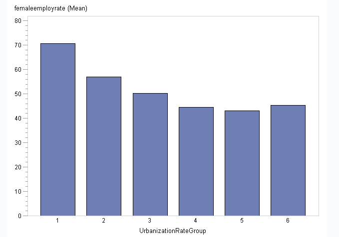
A bar chart reveals an inverse association between female employ rate and the urban rate.

/** TESTING MODERATION IN THE CONTEXT OF CHI SQUARE TEST OF INDEPENDENCE **/

PROC SORT DATA=NEW;

BY IncomePerPersonGroup;

RUN;

PROC FREQ DATA=NEW;    

     TABLES FemaleEmploymentRateGroup * UrbanizationRateGroup / CHISQ; 

BY IncomePerPersonGroup;

RUN;

Results:

The results show an inverse association between the female employ rate and urbanization rate in the first and third income levels, where the income per person are $800 or lower, and between $2,000-$8,000.  At these income levels, the P-values are statistically significant (0.0015 for income level 1 and 0.0087 for income level 3) and have the highest Chi Square values of 44.1 for income level 1 and 26.6 for income level 3. Income levels 2, 4, 5 and 6 have P-values higher than 0.05 and are therefore not statistically significant. 

Testing Statistical Interaction or Moderation In The Context of the Pearson Correlation Coefficient

/** TESTING MODERATION IN THE CONTEXT OF CORRELATION **/

PROC SORT DATA=NEW;

BY IncomePerPersonGroup;

RUN;

PROC CORR DATA=NEW;

VAR urbanrate femaleemployrate;

BY IncomePerPersonGroup;

RUN;

Results:

The results show an inverse association between the female employ rate and urbanization rate in the first income level, where the income per person is $800 or lower. At this income level, the P-value is statistically significant (0.0006) with a correlation co-efficient of -.46785.  Income levels 2,3, 4, 5 and 6 have P-values higher than 0.05 and are therefore not statistically significant. 

Pearson Correlation

Using data from the Gapminder codebook: female employ rate  and urban rate. The data output was generated using SAS Studio.

Hypothesis formulation

Based on research review, it appears that while more women have joined the labor force thanks to urbanization, they have encountered several cultural and social obstacles that have negatively impacted their employment rates. It would be interesting to study the correlation between urbanization and the female employment rate in the Gapminder dataset. Hypothesis: Higher urbanization rates lead to lower female employment rates.

Calculating the Pearson Correlation

code

/** DETERMINING THE CO-EFFICIENT CORRELATION**/

PROC CORR DATA=work.newdata;

          VAR urbanrate femaleemployrate;

RUN;

results:

For the association between urban rate and female employment rate, the correlation co-efficient is approximately -0.303, with p-vale < 0.0001. The association between urban rate and female employment rate appears to be modestly negative and significant statistically . It is therefore unlikely that the association is by chance alone.

Squaring the correlation co-efficient gives us the fraction of the variability of one variable that can be predicted by another. 

R^2 = (-0.303)^2 = 0.091797,

Therefore, if we know the urban rate we can predict approximately 9.2% of the variability we see in the female employment rate. This means that 91% of the variability is due to factors other than the urban rate.

This scatter plot shows the correlation between female employment rate and urban rate:

/** SCATTER PLOT **/
PROC SGPLOT DATA=WORK.NEWDATA;
REG X=urbanrate Y=femaleemployrate;
RUN;

Chi-Square Test of independence

Using data from the Gapminder codebook: female employ rate  and urban rate. The data output was generated using SAS Studio.

Hypothesis formulation

Based on research review, it appears that while more women have joined the labor force thanks to urbanization, they have encountered several cultural and social obstacles that have negatively impacted their employment rates. It would be interesting to study the correlation between urbanization and the female employment rate in the Gapminder dataset.

Hypothesis: Higher urbanization rates lead to lower female employment rates.

Chi-Square Test
A Chi-Square test of independence was used to look for the association or difference between female employment rates and urbanization rates based on the hypothesis being tested. Because there are several continuous values in both variables, the data for each variable was grouped into categories in a previous assignment. The categories were then used in the chi-square test.

SAS Code
/** CHI SQUARE TEST OF INDEPENDENCE **/
PROC FREQ DATA=NEW;   
TABLES FemaleEmploymentRateGroup * UrbanizationRateGroup / CHISQ; 
TITLE 'Chi-Squared Test of Independence: Female Employment Rate and Urbanization Rate';
RUN;

Results
The contingency table shows:
The row percentages (Female Employment Rate Group / response variable) appear to be higher than the column percentages (Urbanization Rate Groups / independent variable) for Female Employment Rate Groups 1, 2, 5 and 6. The reverse is true for rows 3, 4 and 5. The data suggests an inverse relationship between the two groups. The higher level urbanization rate groups appear to have a lower percentage of female employment rates.

The Statistics table shows a Chi-Square value of 52.58 that is significant at the 0.001 probability level. The probability is less than .001 indicating a strong relationship between these two variables.

Post-hoc Tests for Chi Square Tests of Independence

This is used to examine the p-value and protect against a Type 1 error by using the Bonferroni Adjustment. The Null hypothesis will be rejected at the P-value / Comparisons level, i.e. 0.05/15 = 0.003333 

 Below are the Chi Square p-levels generated from pairs of each of the 6 levels in the Urbanization Rate Group. Level 1 has the most number of statistically significant values (below 0.003), for pair-wise comparisons (1,4), (1,5) and (1,6).

SAS Code:

DATA COMPARISON1; 

SET WORK.NEW;    

IF UrbanizationRateGroup = '1' OR UrbanizationRateGroup = '2';

PROC FREQ; 

     TABLES FemaleEmploymentRateGroup * UrbanizationRateGroup / CHISQ; 

RUN;

DATA COMPARISON2; 

SET WORK.NEW;    

IF UrbanizationRateGroup = '1' OR UrbanizationRateGroup = '3';

PROC FREQ; 

     TABLES FemaleEmploymentRateGroup * UrbanizationRateGroup / CHISQ; 

RUN;

DATA COMPARISON3; 

SET WORK.NEW;    

IF UrbanizationRateGroup = '1' OR UrbanizationRateGroup = '4';

PROC FREQ; 

     TABLES FemaleEmploymentRateGroup * UrbanizationRateGroup / CHISQ; 

RUN;

DATA COMPARISON4; 

SET WORK.NEW;    

IF UrbanizationRateGroup = '1' OR UrbanizationRateGroup = '5';

PROC FREQ; 

     TABLES FemaleEmploymentRateGroup * UrbanizationRateGroup / CHISQ; 

RUN;

DATA COMPARISON5; 

SET WORK.NEW;    

IF UrbanizationRateGroup = '1' OR UrbanizationRateGroup = '6';

PROC FREQ; 

     TABLES FemaleEmploymentRateGroup * UrbanizationRateGroup / CHISQ; 

RUN;

DATA COMPARISON6; 

SET WORK.NEW;    

IF UrbanizationRateGroup = '2' OR UrbanizationRateGroup = '3';

PROC FREQ; 

     TABLES FemaleEmploymentRateGroup * UrbanizationRateGroup / CHISQ; 

RUN;

DATA COMPARISON7; 

SET WORK.NEW;    

IF UrbanizationRateGroup = '2' OR UrbanizationRateGroup = '4';

PROC FREQ; 

     TABLES FemaleEmploymentRateGroup * UrbanizationRateGroup / CHISQ; 

RUN;

DATA COMPARISON8; 

SET WORK.NEW;    

IF UrbanizationRateGroup = '2' OR UrbanizationRateGroup = '5';

PROC FREQ; 

     TABLES FemaleEmploymentRateGroup * UrbanizationRateGroup / CHISQ; 

RUN;

DATA COMPARISON9; 

SET WORK.NEW;    

IF UrbanizationRateGroup = '2' OR UrbanizationRateGroup = '6';

PROC FREQ; 

     TABLES FemaleEmploymentRateGroup * UrbanizationRateGroup / CHISQ; 

RUN;

DATA COMPARISON10; 

SET WORK.NEW;    

IF UrbanizationRateGroup = '3' OR UrbanizationRateGroup = '4';

PROC FREQ; 

     TABLES FemaleEmploymentRateGroup * UrbanizationRateGroup / CHISQ; 

RUN;

DATA COMPARISON11; 

SET WORK.NEW;    

IF UrbanizationRateGroup = '3' OR UrbanizationRateGroup = '5';

PROC FREQ; 

     TABLES FemaleEmploymentRateGroup * UrbanizationRateGroup / CHISQ; 

RUN;

DATA COMPARISON12; 

SET WORK.NEW;    

IF UrbanizationRateGroup = '3' OR UrbanizationRateGroup = '6';

PROC FREQ; 

     TABLES FemaleEmploymentRateGroup * UrbanizationRateGroup / CHISQ; 

RUN;

DATA COMPARISON13; 

SET WORK.NEW;    

IF UrbanizationRateGroup = '4' OR UrbanizationRateGroup = '5';

PROC FREQ; 

     TABLES FemaleEmploymentRateGroup * UrbanizationRateGroup / CHISQ; 

RUN;

DATA COMPARISON14; 

SET WORK.NEW;    

IF UrbanizationRateGroup = '4' OR UrbanizationRateGroup = '6';

PROC FREQ; 

     TABLES FemaleEmploymentRateGroup * UrbanizationRateGroup / CHISQ; 

RUN;

DATA COMPARISON15; 

SET WORK.NEW;    

IF UrbanizationRateGroup = '5' OR UrbanizationRateGroup = '6';

PROC FREQ; 

     TABLES FemaleEmploymentRateGroup * UrbanizationRateGroup / CHISQ; 

RUN;

Using PROC ANOVA For One-Way Analysis of Variance

Using data from the Gapminder codebook: female employ rate  and urban rate. The data output was generated using SAS Studio.


Hypothesis formulation

Based on research review, it appears that while more women have joined the labor force thanks to urbanization, they have encountered several cultural and social obstacles that have negatively impacted their employment rates. It would be interesting to study the correlation between urbanization and the female employment rate in the Gapminder dataset. Hypothesis: Higher urbanization rates lead to lower female employment rates.

Summary of findings:

• The “Class Level Information” table lists the variables that appear in the CLASS statement, their levels, and the number of observations in the data set. There are 6 levels, 213 observations read and 173 observations used.
• The model degrees of freedom (DF) for the one-way analysis of variance are the number of levels minus 1; in this case, 6 - 1=5.
• The Corrected Total degrees of freedom are the total number of observations minus one; in this case 173 – 1 = 172. The sum of Model and Error degrees of freedom equal the Corrected Total.
• The overall F test is significant (F = 6.29; p < 0.0001), indicating that the model as a whole accounts for a significant portion of the variability in the female employ rate.
• The F test for the urbanization rate groups is significant, indicating that some contrast between the means for the different urbanization rate groups is different from zero. The null hypothesis is rejected.
• The Model and Urbanization Rate Groups F tests are identical, since “Urbanizationrategroup”  is the only term in the model.

Further analysis:

• The F test for Urbanization Rate Groups (F = 6.29; p < 0.0001) suggests that there are female employ rate distribution rate differences among the urbanization rate groups, but it does not reveal any information about the nature of the differences. A Mean comparison methods is used to gather further information using Tukey’s multiple comparisons test for pairwise differences between the urbanization rate group means.
• Significant differences in the female employ rate are observed between:
• Urbanization rate group 1 and groups 6, 4, and 5
• Urbanization rate group 2 and groups 6, 4, and 5

Code:

/** USING PROC ANOVA FOR ONE-WAY ANALYSIS OF VARIANCE **/

/** PROC ANOVA is used when the independent variable is categorical and the dependent variable is continuous. 

       Independent variable: UrbanizationRateGroup (categorized in the Binning/Grouping assignment)

Dependent: Female employ rate (continuous variable)

**/

PROC ANOVA  DATA=NEW;

CLASS UrbanizationRateGroup; /** defines the categorical variable **/

MODEL femaleemployrate = UrbanizationRateGroup; /** defines the dependent variable  & effects **/  

RUN;

/** Using the TUKEY procedure to further understand differences in the categorical variable **/

PROC ANOVA  DATA=NEW;

CLASS UrbanizationRateGroup; 

MODEL femaleemployrate = UrbanizationRateGroup; 

    MEANS UrbanizationRateGroup / TUKEY;    / ** studentized range test **/

RUN;

Results:

                                                                Urbanization Rate Vertical Bar Chart

The ANOVA Procedure

Class Level Information
Class	Levels	Values
UrbanizationRateGroup	6	1 2 3 4 5 6

Number of Observations Read	213
Number of Observations Used	173

The ANOVA Procedure

Dependent Variable: femaleemployrate

Source	DF	Sum of Squares	Mean Square	F Value	Pr > F
Model	5	5948.15795	1189.63159	6.29	<.0001
Error	167	31599.31337	189.21745
Corrected Total	172	37547.47132

R-Square	Coeff Var	Root MSE	femaleemployrate Mean
0.158417	28.80604	13.75563	47.75260

Source	DF	Anova SS	Mean Square	F Value	Pr > F
UrbanizationRateGrou	5	5948.157954	1189.631591	6.29	<.0001

The ANOVA Procedure

Tukey's Studentized Range (HSD) Test for femaleemployrate

Note:This test controls the Type I experimentwise error rate.

Alpha	0.05
Error Degrees of Freedom	167
Error Mean Square	189.2174
Critical Value of Studentized Range	4.07731

Comparisons significant at the 0.05 level are indicated by ***.
UrbanizationRateGroup Comparison	Difference Between Means	Simultaneous 95% Confidence Limits
1 - 2	13.615	-7.742	34.972
1 - 3	20.462	-0.648	41.572
1 - 6	25.280	4.459	46.102	***
1 - 4	26.208	5.098	47.318	***
1 - 5	27.537	6.845	48.229	***
2 - 1	-13.615	-34.972	7.742
2 - 3	6.847	-3.893	17.586
2 - 6	11.665	1.504	21.826	***
2 - 4	12.593	1.854	23.333	***
2 - 5	13.922	4.030	23.815	***
3 - 1	-20.462	-41.572	0.648
3 - 2	-6.847	-17.586	3.893
3 - 6	4.818	-4.813	14.449
3 - 4	5.747	-4.493	15.987
3 - 5	7.076	-2.272	16.423
6 - 1	-25.280	-46.102	-4.459	***
6 - 2	-11.665	-21.826	-1.504	***
6 - 3	-4.818	-14.449	4.813
6 - 4	0.928	-8.703	10.559
6 - 5	2.257	-6.419	10.934
4 - 1	-26.208	-47.318	-5.098	***
4 - 2	-12.593	-23.333	-1.854	***
4 - 3	-5.747	-15.987	4.493
4 - 6	-0.928	-10.559	8.703
4 - 5	1.329	-8.019	10.677
5 - 1	-27.537	-48.229	-6.845	***
5 - 2	-13.922	-23.815	-4.030	***
5 - 3	-7.076	-16.423	2.272
5 - 6	-2.257	-10.934	6.419
5 - 4	-1.329	-10.677	8.019